Overview
A common challenge in integrative analysis of high-dimensional data sets is subsequent biological interpretation. Anansi addresses this challenge by only considering pairwise associations that are known to occur a priori. In order to achieve this, we need to provide this relational information to anansi in the form of a (bi)adjacency matrix.
This vignette can be divided into two sections:
Understanding adjacency matrices
Example from Biology: The Krebs cycle
Recall that the citric acid cycle, or Krebs cycle, is a central piece of metabolic machinery involved in oxidative phosphorylation. See figure below for a simplified representation with 8 unique enzymatic reactions and 9 unique metabolites.
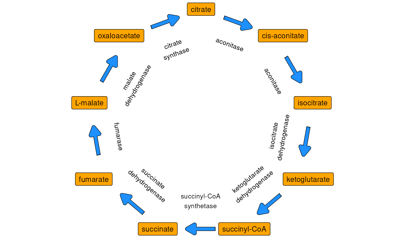
Simplified representation of the Krebs cycle. Orange boxes mark metabolites and blue arrows represent enyzmes.
Adjacency matrices allow us to be specific in our questions
Let’s imagine we had (high-dimensional proxy) measurements available for both types. For instance, we could have transcription data for the enzymes and metabolomics data for the metabolites. We could represent our two data sets like two sets of features.
All vs-all testing
If we were to perform an all-vs-all integrative analysis between our two data sets, comprehensively testing every metabolite-enzyme pair, we’d test \(8\times9=72\) hypotheses.
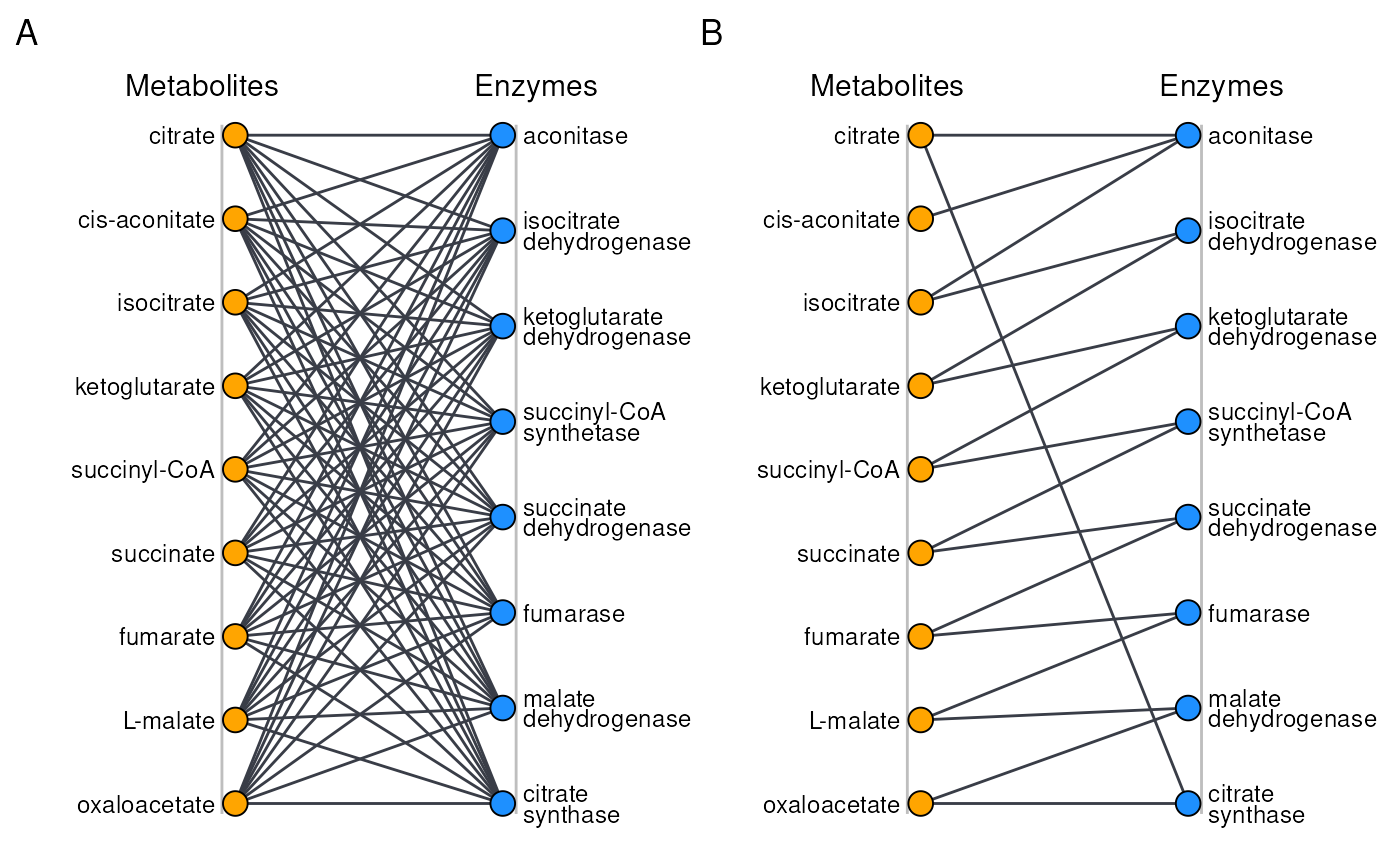
Graph representation of possible association sctructures in the Krebs cycle. A) All-vs-all, with a full graph. B) Constrained, only linking metabolites an enzymes that are known to directly interact.
Knowledge-informed analyis of specific interactions
Often however, only a subset of these comparisons is scientifically relevant to investigate. In this case for instance, only 17 associations between enzyme-metabolite pairs are likely to make sense. Non-selectively testing all 72 associations actively harms statistical power, as 55 of these tests likely cannot be interpreted, but their p-values will still be tallied for the purpose of FDR and FWER. Moreover, they tend to obscure any biologically interpretable findings.
In order to ‘know’ which features-pairs in your data set should be considered, anansi requires a biadjacency matrix. The biadjacency matrix corresponding to to the sparser graph on the right can be seen in the figure below.
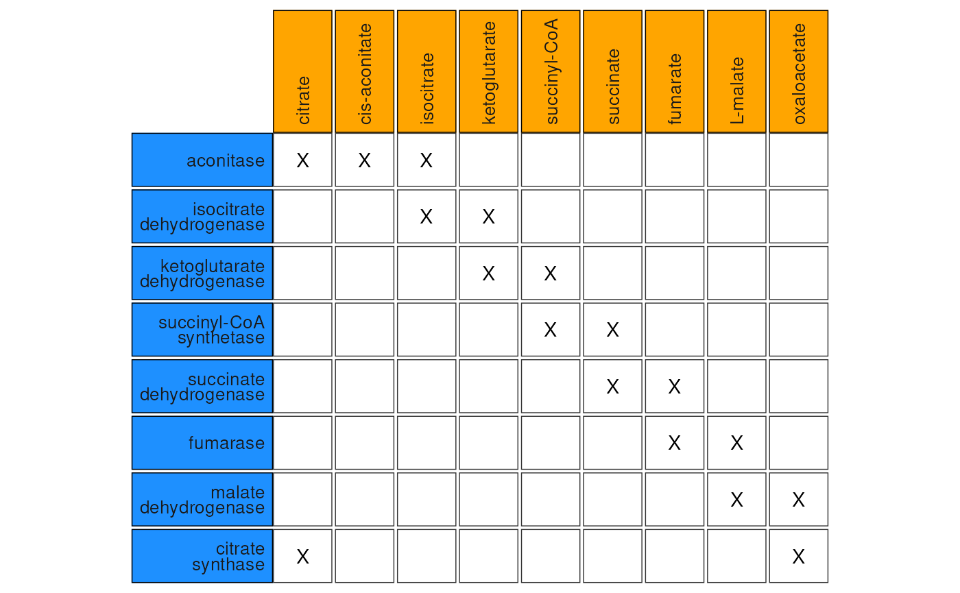
Matrix representation of the constrained analysis of the Krebs cycle, with cells marked with ‘X’ signifying tested feature-pairs.
General use in anansi
In anansi, we work with biadjacency matrices in the
AnansiWeb S7 class, which consists of a biadjacency matrix,
in this case we call it a dictionary, as well as two tables
of observations that should be analysed jointly.
The anansi package offers some functions that should be sufficient for basic analysis. To enable more advanced users to pursue non-standard applications, our methodology is compatible with several popular interfaces.
Make a biadjacency matrix with weaveWeb()
The recommended default interface to generate an
AnansiWeb object is weaveWeb(). Besides a
traditional interface, it also accepts R formula syntax.
Once we have an AnansiWeb object, we can use the $ operator
to access the biadjacency matrix in the ‘dictionary’ slot.
## Warning in .check_metadata_labels(metadata, tableY, tableX): Argument
## `metadata` not provided; Please validate sample ID order.## Warning in .check_metadata_labels(metadata, tableY, tableX): Argument
## `metadata` not provided; Please validate sample ID order.
# Same output
identical(form.web, trad.web)## [1] TRUE
# Get the biadjacency matrix using the $ operator
head(dictionary(form.web), c(10, 10))## 10 x 10 sparse Matrix of class "ngCMatrix"## [[ suppressing 10 column names 'K00001', 'K00002', 'K00003' ... ]]## ko
## ec
## 1.1.1.1 | . . . . . . . . .
## 1.1.1.2 . | . . . . . . . .
## 1.1.1.3 . . | . . . . . . .
## 1.1.1.4 . . . | . . . . . .
## 1.1.1.303 . . . | . . . . . .
## 1.1.1.6 . . . . | . . . . .
## 1.1.1.8 . . . . . | . . . .
## 1.1.1.11 . . . . . . | . . .
## 1.1.1.14 . . . . . . . | . .
## 1.1.1.17 . . . . . . . . | .Note that the majority of this matrix consists of dots, it’s a sparse matrix, which is a format that can considerably speed up calculations involving huge, mostly empty matrices. For further reading, see the Matrix package website.
weaveWeb() input: link
weaveWeb() takes additional arguments, let’s focus on
link, which will take the information necessary to link
features between input data sets. The anansi package includes such data
for the KEGG database, let’s
take a look at some of it:
# Extract the data.frame from the list that kegg_link() returns
ec2ko <- kegg_link()[["ec2ko"]]
head(ec2ko)## ec ko
## 1 1.1.1.1 K00001
## 2 1.1.1.2 K00002
## 3 1.1.1.3 K00003
## 4 1.1.1.4 K00004
## 5 1.1.1.303 K00004
## 6 1.1.1.6 K00005Structure of link input
The format of the data.frame is important: It should
have two named columns. Each column contains feature IDs of one type (in
this case, ec and ko, which is how the KEGG
database refers to Enzyme
Commission numbers and kegg orthologes,
respectively. If two feature IDs are on the same row of the
data.frame, it means those features are paired (hence
adjacency).
linking between feature names
The column names correspond to the types of feature IDs that should
be linked. These names are used throughout the AnansiWeb
workflow. They can be directly called from an AnansiWeb
object:
## Warning in .check_metadata_labels(metadata, tableY, tableX): Argument
## `metadata` not provided; Please validate sample ID order.## [1] "ko" "ec"## Warning in .check_metadata_labels(metadata, tableY, tableX): Argument
## `metadata` not provided; Please validate sample ID order.## [1] "ec" "ko"The pre-packaged kegg linking map
We need to provide weaveWeb() with a map of which
features are linked. We can use the pre-packaged kegg link map, which
consists of two similarly structured data.frames in a list,
one of which we just inspected. We can call it directly using
kegg_link():
## $ec2ko
##          ec     ko
## 1   1.1.1.1 K00001
## 2   1.1.1.2 K00002
## 3   1.1.1.3 K00003
## 4   1.1.1.4 K00004
## 5 1.1.1.303 K00004
## 6   1.1.1.6 K00005
##
## $ec2cpd
## ec cpd
## 1 1.1.1.1 C00001
## 2 1.1.1.115 C00001
## 3 1.1.1.132 C00001
## 4 1.1.1.136 C00001
## 5 1.1.1.170 C00001
## 6 1.1.1.186 C00001linking across two data.frame
Note the column names in the two data.frames:
ec, cpd and ko. Two of these
correspond to the formula we used just used:
weaveWeb(ec ~ ko). We didn’t use the term cpd.
Further, ec is present in both
data.frames.
We can use weaveWeb() to make a biadjacency matrix
between any combination of one or two similarly structured
data.frames, presented as a list. For the pre- packaged
data set, this means we can link between any two of ec,
cpd and ko, in either order.
# Formula notation
head(dictionary(weaveWeb(cpd ~ ko, link = kegg_link())), c(10, 10))
## Warning in .check_metadata_labels(metadata, tableY, tableX): Argument
## `metadata` not provided; Please validate sample ID order.## 10 x 10 sparse Matrix of class "ngCMatrix"## [[ suppressing 10 column names 'K00001', 'K00002', 'K00003' ... ]]## ko
## cpd
## C00001 | . . . . . . . . .
## C00002 . . . . . . . . . .
## C00003 | . | | | | | | | |
## C00004 | . | | | | | | | |
## C00005 | | | . . . . . . .
## C00006 | | | . . . . . . .
## C00007 . . . . . . . . . .
## C00008 . . . . . . . . . .
## C00009 . . . . . . . . . .
## C00010 . . . . . . . . . .
# Character notation
head(dictionary(weaveWeb(y = "ko", x = "cpd", link = kegg_link())), c(10, 10))
## Warning in .check_metadata_labels(metadata, tableY, tableX): Argument
## `metadata` not provided; Please validate sample ID order.## 10 x 10 sparse Matrix of class "ngCMatrix"## [[ suppressing 10 column names 'C00001', 'C00002', 'C00003' ... ]]## cpd
## ko
## K00001 | . | | | | . . . .
## K00002 . . . . | | . . . .
## K00003 . . | | | | . . . .
## K00004 . . | | . . . . . .
## K00005 . . | | . . . . . .
## K00006 . . | | . . . . . .
## K00007 . . | | . . . . . .
## K00008 . . | | . . . . . .
## K00009 . . | | . . . . . .
## K00010 . . | | . . . . . .Use custom biadjacency matrices with AnansiWeb()
The most flexible way to make an AnansiWeb object is
through AnansiWeb():
# Prep some dummy input tables
tX <- matrix(rnorm(30), nrow = 6, dimnames = list(NULL, x = paste("x", seq_len(5),
    sep = "_")))
tY <- matrix(rnorm(42), nrow = 6, dimnames = list(NULL, y = paste("y", seq_len(7),
    sep = "_")))

# Prep biadjacency matrix base::matrix is fine too, but will get coerced to
# Matrix::Matrix.
d <- matrix(data = sample(x = c(TRUE, FALSE), size = 35, replace = TRUE), nrow = NCOL(tY),
    ncol = NCOL(tX), dimnames = list(colnames(tY), colnames(tX)))

# make the AnansiWeb
w <- AnansiWeb(tableY = tY, tableX = tX, dictionary = d)
## Warning in AnansiWeb(tableY = tY, tableX = tX, dictionary = d): Dimnames of
## 'dictionary' were missing; Assigned 'y' and 'x'.## Warning in .check_metadata_labels(metadata, tableY, tableX): Argument
## `metadata` not provided; Please validate sample ID order.
# Confirm the warning:
names(w)
## [1] "y" "x"Additional approaches
There are numerous ways in which we can define an adjacency matrix. Here, we demonstrate a graph-based and matrix based approach.
adjacency matrices with igraph
Importantly, (bi)adjacency matrices can be understood as graphs. Two
common packages that deal with graphs are igraph and graph.
To start off, we need to have a graph object, so let’s make one using
igraph.
##                        Enzyme    Metabolite
## 1    isocitrate dehydrogenase    isocitrate
## 2    isocitrate dehydrogenase ketoglutarate
## 3 ketoglutarate dehydrogenase ketoglutarate
## 4 ketoglutarate dehydrogenase  succinyl-CoA
## 5     succinyl-CoA synthetase  succinyl-CoA
## 6     succinyl-CoA synthetase     succinate
# Convert data.frame to graph
g <- graph_from_data_frame(krebs_edge_df, directed = FALSE)
Now that we have constructed a graph, we still need to identify which
features, vertices, belong to which data modality, in this case either
enzymes and metabolites. Using the igraph package, this
should be done through the type slot. type can
be assigned a boolean vector, where TRUE values become
columns, corresponding to features in tableX, whereas
FALSE values become rows, which correspond to those in
tableY.
V(g)$type <- V(g)$name %in% krebs_edge_df$Metabolite

# Now that we've defined type, we can convert to biadjacency matrix:
bi_mat1 <- as_biadjacency_matrix(g, sparse = TRUE)


head(bi_mat1, n = c(4, 5))
## 4 x 5 sparse Matrix of class "dgTMatrix"
## isocitrate ketoglutarate succinyl-CoA succinate
## isocitrate dehydrogenase 1 1 . .
## ketoglutarate dehydrogenase . 1 1 .
## succinyl-CoA synthetase . . 1 1
## succinate dehydrogenase . . . 1
## fumarate
## isocitrate dehydrogenase .
## ketoglutarate dehydrogenase .
## succinyl-CoA synthetase .
## succinate dehydrogenase 1Though biadjacency support in graph is currently
limited, We note that igraph and graph objects can be converted using
the graph_from_graphnel() and as_graphnel()
functions in igraph.
adjacency matrices with Matrix
We can also define a matrix directly. Conveniently, sparse matrices
can be defined easily from our starting data. The Matrix
library provides fantastic support for this.
library(Matrix)

# For this approach, it's useful to prepare the input as two factors:
Enzyme <- factor(krebs_edge_df$Enzyme)
Metabolite <- factor(krebs_edge_df$Metabolite)

# We can get integers out of factors, corresponding to their level indices
bi_mat2 <- sparseMatrix(i = as.integer(Enzyme), j = as.integer(Metabolite), dimnames = list(Enzyme = levels(Enzyme),
    Metabolite = levels(Metabolite)))

head(bi_mat2, n = c(4, 5))
## 4 x 5 sparse Matrix of class "ngCMatrix"
## Metabolite
## Enzyme citrate cis-aconitate isocitrate ketoglutarate
## aconitase | | | .
## isocitrate dehydrogenase . . | |
## ketoglutarate dehydrogenase . . . |
## succinyl-CoA synthetase . . . .
## Metabolite
## Enzyme succinyl-CoA
## aconitase .
## isocitrate dehydrogenase .
## ketoglutarate dehydrogenase |
## succinyl-CoA synthetase |Session info
## R version 4.5.1 (2025-06-13)
## Platform: x86_64-pc-linux-gnu
## Running under: Ubuntu 24.04.3 LTS
##
## Matrix products: default
## BLAS:   /usr/lib/x86_64-linux-gnu/openblas-pthread/libblas.so.3
## LAPACK: /usr/lib/x86_64-linux-gnu/openblas-pthread/libopenblasp-r0.3.26.so;  LAPACK version 3.12.0
##
## locale:
##  [1] LC_CTYPE=en_US.UTF-8       LC_NUMERIC=C
##  [3] LC_TIME=en_US.UTF-8        LC_COLLATE=en_US.UTF-8
##  [5] LC_MONETARY=en_US.UTF-8    LC_MESSAGES=en_US.UTF-8
##  [7] LC_PAPER=en_US.UTF-8       LC_NAME=C
##  [9] LC_ADDRESS=C               LC_TELEPHONE=C
## [11] LC_MEASUREMENT=en_US.UTF-8 LC_IDENTIFICATION=C
##
## time zone: UTC
## tzcode source: system (glibc)
##
## attached base packages:
## [1] stats     graphics  grDevices utils     datasets  methods   base
##
## other attached packages:
## [1] Matrix_1.7-4     dplyr_1.1.4      tidygraph_1.3.1  igraph_2.1.4
## [5] ggraph_2.2.2     patchwork_1.3.2  ggplot2_4.0.0    anansi_0.99.4
## [9] BiocStyle_2.37.1
##
## loaded via a namespace (and not attached):
##  [1] tidyselect_1.2.1                viridisLite_0.4.2
##  [3] farver_2.1.2                    viridis_0.6.5
##  [5] Biostrings_2.77.2               S7_0.2.0
##  [7] fastmap_1.2.0                   SingleCellExperiment_1.31.1
##  [9] lazyeval_0.2.2                  tweenr_2.0.3
## [11] digest_0.6.37                   lifecycle_1.0.4
## [13] tidytree_0.4.6                  magrittr_2.0.4
## [15] compiler_4.5.1                  rlang_1.1.6
## [17] sass_0.4.10                     tools_4.5.1
## [19] yaml_2.3.10                     knitr_1.50
## [21] labeling_0.4.3                  graphlayouts_1.2.2
## [23] S4Arrays_1.9.1                  htmlwidgets_1.6.4
## [25] DelayedArray_0.35.3             RColorBrewer_1.1-3
## [27] TreeSummarizedExperiment_2.17.1 abind_1.4-8
## [29] BiocParallel_1.43.4             withr_3.0.2
## [31] purrr_1.1.0                     BiocGenerics_0.55.3
## [33] desc_1.4.3                      grid_4.5.1
## [35] polyclip_1.10-7                 stats4_4.5.1
## [37] scales_1.4.0                    MASS_7.3-65
## [39] MultiAssayExperiment_1.35.9     SummarizedExperiment_1.39.2
## [41] cli_3.6.5                       rmarkdown_2.30
## [43] crayon_1.5.3                    ragg_1.5.0
## [45] treeio_1.33.0                   generics_0.1.4
## [47] BiocBaseUtils_1.11.2            ape_5.8-1
## [49] cachem_1.1.0                    ggforce_0.5.0
## [51] parallel_4.5.1                  formatR_1.14
## [53] BiocManager_1.30.26             XVector_0.49.1
## [55] matrixStats_1.5.0               vctrs_0.6.5
## [57] yulab.utils_0.2.1               jsonlite_2.0.0
## [59] bookdown_0.45                   IRanges_2.43.5
## [61] S4Vectors_0.47.4                ggrepel_0.9.6
## [63] systemfonts_1.3.1               jquerylib_0.1.4
## [65] tidyr_1.3.1                     glue_1.8.0
## [67] pkgdown_2.1.3                   codetools_0.2-20
## [69] gtable_0.3.6                    GenomicRanges_1.61.5
## [71] tibble_3.3.0                    pillar_1.11.1
## [73] rappdirs_0.3.3                  htmltools_0.5.8.1
## [75] Seqinfo_0.99.2                  R6_2.6.1
## [77] textshaping_1.0.3               evaluate_1.0.5
## [79] lattice_0.22-7                  Biobase_2.69.1
## [81] memoise_2.0.1                   bslib_0.9.0
## [83] Rcpp_1.1.0                      gridExtra_2.3
## [85] SparseArray_1.9.1               nlme_3.1-168
## [87] xfun_0.53                       fs_1.6.6
## [89] MatrixGenerics_1.21.0           forcats_1.0.1
## [91] pkgconfig_2.0.3